Introduction to Gaussian Splatting

1. Introduction to Gaussian Splatting

When it comes to radiance field rendering, a relatively recent yet effective technique stands out for its innovative approach to depicting complex scenes with remarkable efficiency and realism: Gaussian Splatting [1]. At its core, Gaussian Splatting represents a leap forward in how we project and blend information from three-dimensional points onto a two-dimensional image plane, leveraging the mathematical principles of Gaussian functions. This technique is instrumental in rendering scenes laden with intricate details, achieving an unprecedented level of smoothness and visual fidelity.

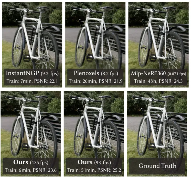
The genesis of Gaussian Splatting can be traced back to the foundational work on Neural Radiance Fields (NeRFs) [5], a paradigm-shifting framework that has revolutionized our ability to create photorealistic images from sparse data sets. NeRFs employ deep learning to interpolate and render complex scenes by understanding the spatial distribution of light and color in 3D space. Gaussian Splatting builds upon this framework, offering a method that not only complements but significantly enhances the rendering process. Through its efficient simulation of light interactions with surfaces, Gaussian Splatting enables the creation of images that are not just visually appealing but are also computationally feasible, even in scenes of daunting complexity.

The essence of Gaussian Splatting lies in its ability to smooth out the projection of information—such as color and density—from 3D points to the 2D plane using Gaussian functions. This smoothing is crucial for eliminating the harsh edges and artifacts that commonly plague rendered images, thereby ensuring a more natural and cohesive visual experience. By applying this technique, researchers have achieved levels of detail and realism previously unattainable, opening new vistas in the fields of virtual reality, game development, and cinematic visual effects [2][3][4].

Furthermore, the application of Gaussian Splatting extends beyond mere image enhancement. It represents a significant step forward in computational photography and visualization, enabling the reconstruction of scenes from real-world data with an accuracy and depth that were once out of reach. This has profound implications not just for entertainment and media but also for areas such as architectural visualization, digital heritage preservation, and even medical imaging, where the detailed and realistic representation of complex structures is paramount.

As we delve deeper into the mechanics and applications of Gaussian Splatting, it’s essential to acknowledge the pioneering studies and papers that laid the groundwork for this technique. The original paper on Neural Radiance Fields by Mildenhall et al. [5] introduced the world to the potential of deep learning in rendering, setting the stage for subsequent innovations like Gaussian Splatting. Further developments and explorations into this technique [8][6][7] have continued to push the boundaries of what’s possible, highlighting the collaborative effort of the scientific community in advancing our understanding and capabilities in computer graphics.

2. Mathematical Foundations of Gaussian Splatting

Gaussian Splatting is predicated on the principle of projecting information from a three-dimensional point cloud onto a two-dimensional plane. This section will elucidate the key mathematical constructs that govern this process.

2.1 Gaussian Distribution in Splatting

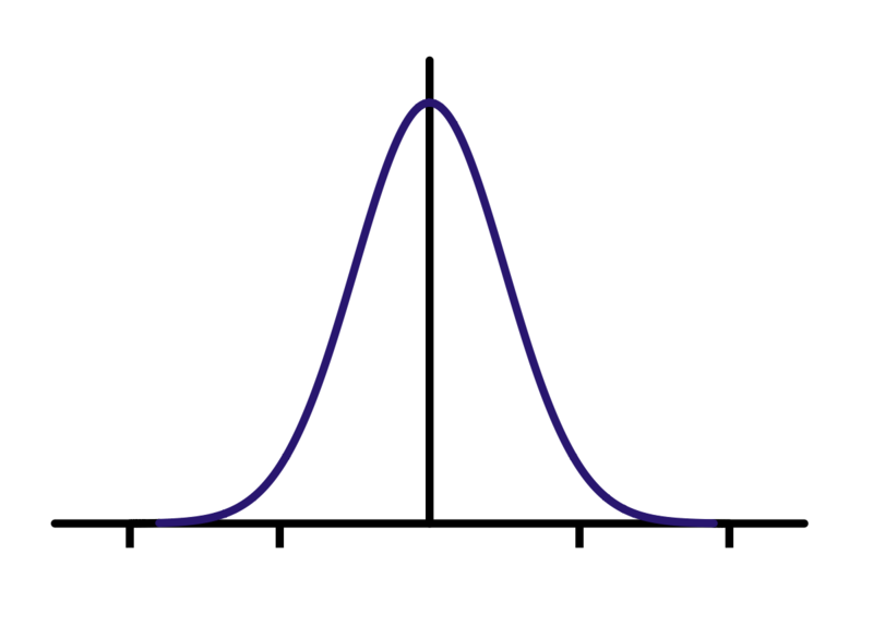
At the core of Gaussian Splatting is the Gaussian distribution function, which is instrumental in the spatial blending of points. The Gaussian distribution, defined as follows, ensures a smooth gradient of influence around a point’s location:

\[ G(x) = \frac{1}{\sigma\sqrt{2\pi}}e^{-\frac{1}{2}(\frac{x-\mu}{\sigma})^2} \quad (1) \]

Here, \(x\) represents the distance from the center of the point, \(\mu\) is the mean or center of the distribution, and \(\sigma\) is the standard deviation that dictates the spread of the distribution.

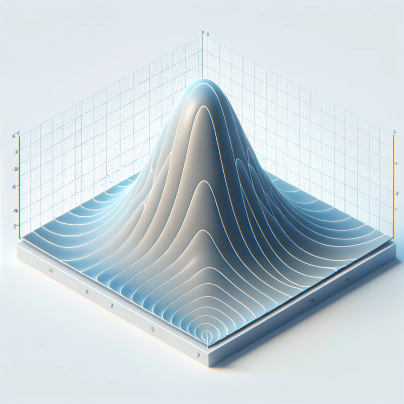
2.2 3D Gaussian Function

Generalizing to 3D space, the core of our technique is a 3D Gaussian function, represented as follows:

\[ G(x) = e^{-\frac{1}{2}(x-\mu)^T\Sigma^{-1}(x-\mu)} \quad (2) \]

where \(\mu\) is the point of interest (mean) and \(\Sigma\) is the covariance matrix in world space, defining the distribution’s spread.

2.3 Rendering Equation with Gaussian Influence

The rendering of an image via Gaussian Splatting can be described by an integral that accumulates the color contributions of each point, modulated by their Gaussian influence and the scene’s opacity at each location:

\[ I(x) = \int_{\mathbb{R}^3} G(|x - p_i|)L(p_i,\omega)V(p_i)dA(p_i) \quad (3) \]

In this equation, \(I(x)\) denotes the intensity at the pixel location \(x\), \(G\) is the Gaussian distribution, \(p_i\) is the position of the i-th point, \(L(p_i,\omega)\) is the radiance from \(p_i\) in direction \(\omega\), and \(V(p_i)\) signifies the visibility function at \(p_i\).

2.4 Opacity and Color Blending

The interplay of light and material properties is captured through the blending of color and opacity. Gaussian Splatting achieves this by overlapping the contributions from different points, accounting for their respective opacities:

\[ C(x) = \frac{\int_{\mathbb{R}^3} G(|x - p_i|)C(p_i)\tau(p_i)dA(p_i)}{\int_{\mathbb{R}^3} G(|x - p_i|)\tau(p_i)dA(p_i)} \quad (4) \]

\(C(x)\) is the resulting color at the pixel location \(x\), \(C(p_i)\) is the color contribution from the i-th point, and \(\tau(p_i)\) represents the opacity at \(p_i\). The denominator ensures normalization of the weighted color contributions, facilitating the correct intensity and hue for the rendered image.

2.5 Projection to 2D Space

For rendering in 2D, a projection of these 3D Gaussians is required. This is achieved by transforming the 3D covariance matrix \(\Sigma\) to camera coordinates:

\[ \Sigma’ = J W \Sigma W^T J^T \quad (5) \]

Here, \(W\) represents the viewing transformation, and \(J\) is the Jacobian of the affine approximation to the projective transformation.

2.6 Ellipsoid Configuration

An ellipsoid’s configuration, offering an intuitive representation for \(\Sigma\), is defined by:

\[ \Sigma = RSS^TR^T \quad (6) \]

where \(S\) is a scaling matrix and \(R\) is a rotation matrix.

3. Kickstart Your Gaussian Splatting Adventure: Setting the Stage with Python

Hey there! Ready to dive into the world of Gaussian Splatting? Let’s get our hands dirty with some code. First things first, we need to gather our tools. Think of this step like packing your bag before a hike. You wouldn’t want to forget your water bottle, right? Similarly, we can’t start without importing some essential Python libraries that will help us on this journey.

What’s in Our Toolkit?

Here’s a sneak peek at the Python goodies we’re bringing along:

import copy
import ipywidgets
import json
import kaolin
import matplotlib.pyplot as plt
import numpy as np
import os
import torch
import torchvision

# And don't forget about our special gear for Gaussian Splatting
from utils.graphics_utils import focal2fov
from utils.system_utils import searchForMaxIteration
from gaussian_renderer import render, GaussianModel
from scene.cameras import Camera as GSCamera

Breaking it down: We’ve got our classic friends like numpy for all things numbers, matplotlib.pyplot to plot our adventures, and torch because, well, neural networks are cool. Kaolin is a bit of a Swiss Army knife for 3D deep learning, so that’s handy!

And those special tools at the bottom? They’re our secret sauce for making Gaussian Splatting magic happen. We’ll dive deeper into those as we move along. But for now, just know that they’re like our map and compass in the wild world of rendering.

One more thing: Ever felt lost looking at tensor dimensions? Well, fear not! We’ve got a little helper function that’s like our very own guide in the tensor jungle:

def log_tensor(t, name, **kwargs):
    print(kaolin.utils.testing.tensor_info(t, name=name, **kwargs))

This handy function will shout out everything we need to know about our tensors, making sure we’re always on the right path.

And that’s it for our prep work! With our bag packed full of Python tools, we’re ready to tackle the exciting world of Gaussian Splatting. Stay tuned for our next step, where we’ll start the actual journey and see these tools in action!

4. Loading the Model

Alright, adventurers! Now that we’ve got our tools, it’s time to summon our magic wand—the checkpoint. This is where our previously trained model lies in wait, full of learned wisdom and ready to splat Gaussians like a pro.

def load_checkpoint(model_path, sh_degree=3, iteration=-1):
    # Magical incantations to find and awaken the checkpoint
    checkpt_dir = os.path.join(model_path, "point_cloud")
    if iteration == -1:
        iteration = searchForMaxIteration(checkpt_dir)
    checkpt_path = os.path.join(checkpt_dir, f"iteration_{iteration}", "point_cloud.ply")
    
    # Awaken the Gaussians from their slumber
    gaussians = GaussianModel(sh_degree)
    gaussians.load_ply(checkpt_path)                                                 
    return gaussians

This spell (function, if you’re not into the whole magic thing) awakens our model, readying it for the adventures ahead. It seeks out the most recent training session if you don’t specify one, ensuring we’re always using the freshest of magical essences.

5. Camera Setup

In any good adventure, knowing where to look is half the battle. That’s why we scry (or load) the perfect camera settings to capture our scene just right.

def try_load_camera(model_path):
    # Attempt to find the mystical eye (camera settings)
    cam_path = os.path.join(model_path, 'cameras.json')
    if not os.path.exists(cam_path):
        print(f'Could not find saved cameras for the scene; using default.')
        # Default camera spell
        return GSCamera(...)
        
    with open(cam_path) as f:
        data = json.load(f)
        # Camera transformation incantations
        ...
    return GSCamera(...)

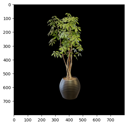
6. Rendering the Scene

Now, let’s pull the curtain back and reveal the magic of our scene. Here’s how we bring a 3D model into the spotlight of our 2D world. We’ll take our camera settings, the mystical Gaussian model, and the background of deep space (just a fancy way of saying a black background) to render our scene.

# The spell to conjure the image
render_res = render(test_camera, gaussians, pipeline, background)
rendering = render_res["render"]

# Let's see what the oracle (our render function) has to say about our render
for k in render_res.keys():
    log_tensor(render_res[k], k, print_stats=True)

# And for the grand finale, let's reveal the image to the world!
plt.imshow((rendering.permute(1, 2, 0) * 255).to(torch.uint8).detach().cpu().numpy())

7. The Art of Camera Conversion

7.1 Calculating the Field of View

To understand our digital realm’s extent, we start by crafting a spell for the field of view (FoV):

def compute_cam_fov(intrinsics, axis='x'):
    # Compute FOV from camera focal length
    aspectScale = intrinsics.width / 2.0
    tanHalfAngle = aspectScale / (intrinsics.focal_x if axis == 'x' else intrinsics.focal_y).item()
    fov = np.arctan(tanHalfAngle) * 2
    return fov

7.2 Morphing Cameras Between Realms

The following incantations allow us to morph our view between the Kaolin and GS realms:

def convert_kaolin_camera(kal_camera):
    # Convert Kaolin camera to GS camera
    R = kal_camera.extrinsics.R[0]
    R[1:3] = -R[1:3] # Invert certain axes
    T = kal_camera.extrinsics.t.squeeze()
    T[1:3] = -T[1:3] # Invert certain axes
    return GSCamera(colmap_id=0,
                    R=R.transpose(1, 0).cpu().numpy(), 
                    T=T.cpu().numpy(), 
                    FoVx=compute_cam_fov(kal_camera.intrinsics, 'x'), 
                    FoVy=compute_cam_fov(kal_camera.intrinsics, 'y'), 
                    image=torch.zeros((3, kal_camera.height, kal_camera.width)), 
                    gt_alpha_mask=None,
                    image_name='fake',
                    uid=0)

def convert_gs_camera(gs_camera):
    # Convert GS camera to Kaolin camera
    view_mat = gs_camera.world_view_transform.transpose(1, 0)
    view_mat[1:3] = -view_mat[1:3] # Invert certain axes
    res = kaolin.render.camera.Camera.from_args(
        view_matrix=view_mat,
        width=gs_camera.image_width, height=gs_camera.image_height,
        fov=gs_camera.FoVx, device='cpu')
    return res

7.3 Ensuring Consistency in Our Rendered Reality

Finally, we cast a spell to ensure the transformed camera views the world just as our original did:

# Test the camera conversion by rendering an image
kal_cam = convert_gs_camera(test_camera)
test_cam_back = convert_kaolin_camera(kal_cam)
rendering = render(test_cam_back, gaussians, pipeline, background)["render"]
plt.imshow((rendering.permute(1, 2, 0) * 255).to(torch.uint8).detach().cpu().numpy())

8. Crafting the Interactive Viewing Spell

With the scene set and our camera converted, it’s time to craft an interactive spell that lets us explore our Gaussian Splatting scene with the ease of a sorcerer’s touch.

8.1 Rendering for Interactivity

We’ll define a rendering function that can accept a Kaolin camera. This bit of magic lets us switch perspectives at will:

def render_kaolin(kaolin_cam):
    # Convert the Kaolin camera to a GS camera
    cam = convert_kaolin_camera(kaolin_cam)
    # Render the scene using the GS camera
    render_res = render(cam, gaussians, pipeline, background)
    # Prepare the image for visualization
    rendering = render_res["render"]
    return (rendering.permute(1, 2, 0) * 255).to(torch.uint8).detach().cpu()

8.2 Setting the Stage for Exploration

We pinpoint the focus of our virtual camera onto our scene. This will be the center of rotation for our interactive viewer:

# Determine the point in space our camera will focus on
focus_at = (kal_cam.cam_pos() - 4. * kal_cam.extrinsics.cam_forward()).squeeze()
# Set up the interactive visualizer with the Kaolin camera
visualizer = kaolin.visualize.IpyTurntableVisualizer(
    512, 512, copy.deepcopy(kal_cam), render_kaolin, 
    focus_at=focus_at, world_up_axis=2, max_fps=12)
# Display the interactive scene
visualizer.show()

With this incantation complete, you should now see a window to your 3D world, ready to be explored with the drag of a mouse or the swipe of a finger. Rotate it, zoom in, and let the details of your creation come to life. Enjoy the magic at your fingertips!

8.3 A Touch of Control: Interactive Viewer Enhancements

With our scene set, let’s add a touch of interactivity that allows us to filter and inspect our Gaussian splats with precision.

8.3.1 Peering Into the Scales

We’ll start by examining the scales of our Gaussians to understand their influence on our rendered scene:

# Investigate the scales of our Gaussians
log_tensor(gaussians.get_scaling, 'scaling after activation', print_stats=True)
log_tensor(gaussians._scaling, 'scaling, raw', print_stats=True)

8.3.2 Selective Rendering Incantation

Next, we conjure up a selective render function that lets us filter Gaussians based on their scale, which is controlled by a mystical slider:

def selective_render_kaolin(kaolin_cam):
    # Filter the Gaussians by their scale using a slider value
    scaling = gaussians._scaling.max(dim=1)[0]
    mask = scaling < slider.value
    # Create a temporary Gaussian model with the filtered splats
    tmp_gaussians = GaussianModel(gaussians.max_sh_degree)
    # Apply the mask to all Gaussian parameters
    tmp_gaussians._xyz = gaussians._xyz[mask, :]
    tmp_gaussians._features_dc = gaussians._features_dc[mask, ...]
    tmp_gaussians._features_rest = gaussians._features_rest[mask, ...]
    tmp_gaussians._opacity = gaussians._opacity[mask, ...]
    tmp_gaussians._scaling = gaussians._scaling[mask, ...]
    tmp_gaussians._rotation = gaussians._rotation[mask, ...]
    tmp_gaussians.active_sh_degree = gaussians.max_sh_degree
    # Render the scene with the filtered Gaussians
    cam = convert_kaolin_camera(kaolin_cam)
    render_res = render(cam, tmp_gaussians, pipeline, background)
    rendering = render_res["render"]
    return (rendering.permute(1, 2, 0) * 255).to(torch.uint8).detach().cpu()

8.3.3 Slider Charm

The following code creates a slider to dynamically adjust the Gaussian filter, re-rendering the scene as the slider moves:

def handle_slider(e):
    # Clear the current output and update the rendering
    visualizer.out.clear_output()
    with visualizer.out:
        visualizer.render_update()

# The slider that controls the Gaussian scale threshold
scaling = gaussians._scaling.max(dim=1)[0]
slider = ipywidgets.FloatSlider(value=scaling.max().item(),
    min=scaling.min().item(), max=scaling.max().item(),
    step=0.1,
    description='Max scale:',
    disabled=False,
    continuous_update=True,
    orientation='horizontal',
    readout=True,
    readout_format='.3f',
)
slider.observe(handle_slider, names='value')

8.3.4 Conjuring the Visualizer and Slider

Finally, we bring forth the interactive visualizer with our selective render function and attach the slider to it:

# Initialize the visualizer with the selective render function
visualizer = kaolin.visualize.IpyTurntableVisualizer(
    512, 512, copy.deepcopy(kal_cam), selective_render_kaolin, 
    focus_at=focus_at, world_up_axis=2, max_fps=12)
# Update the rendering to apply the initial filter from the slider
visualizer.render_update()
# Display the visualizer and the slider for interactive control
display(visualizer.canvas, visualizer.out, slider)

With the slider in place, you now wield the power to filter and scrutinize your scene. Slide through the scales and watch as your Gaussians obey, revealing the fine-tuned beauty of your creation.

References

[1] Kerbl, B., Kopanas, G., Leimkühler, T., & Drettakis, G. (2023). 3D Gaussian Splatting for Real-Time Radiance Field Rendering. ACM Transactions on Graphics, 42(4).

[2] Xiong, H., Muttukuru, S., Upadhyay, R., Chari, P., & Kadambi, A. (2023). SparseGS: Real-Time 360° Sparse View Synthesis using Gaussian Splatting. Arxiv.

[3] Yan, C., Qu, D., Wang, D., Xu, D., Wang, Z., Zhao, B., & Li, X. (2023). GS-SLAM: Dense Visual SLAM with 3D Gaussian Splatting. ArXiv.

[4] Tang, J., Chen, Z., Chen, X., Wang, T., Zeng, G., & Liu, Z. (2024). LGM: Large Multi-View Gaussian Model for High-Resolution 3D Content Creation. arXiv preprint arXiv:2402.05054.

[5] Mildenhall, B., Srinivasan, P. P., Tancik, M., Barron, J. T., Ramamoorthi, R., & Ng, R. (2020). NeRF: Representing Scenes as Neural Radiance Fields for View Synthesis. ECCV.

[6] Yan, Y., Lin, H., Zhou, C., Wang, W., Sun, H., Zhan, K., Lang, X., Zhou, X., & Peng, S. (2024). Street Gaussians for Modeling Dynamic Urban Scenes. arXiv preprint arXiv:2401.01339.

[7] Li, M., Yao, S., Xie, Z., & Chen, K. (2024). GaussianBody: Clothed Human Reconstruction via 3D Gaussian Splatting. ArXiv.

[8] Duan, Y., Wei, F., Dai, Q., He, Y., Chen, W., & Chen, B. (2024). 4D Gaussian Splatting: Towards Efficient Novel View Synthesis for Dynamic Scenes. arXiv preprint arXiv:2402.03307.